H3-Pandas Intro
[ ]:
pip install h3pandas
[1]:
import pandas as pd
import matplotlib.pyplot as plt
import h3pandas
Fetch data
We will use the NYC Taxi dataset for this demo
[2]:
# Download and subset data
df = pd.read_csv('https://github.com/uber-web/kepler.gl-data/raw/master/nyctrips/data.csv')
df = df.rename({'pickup_longitude': 'lng', 'pickup_latitude': 'lat'}, axis=1)[['lng', 'lat', 'passenger_count']]
Only use the central part of the data
[3]:
qt = 0.1
df = df.loc[(df['lng'] > df['lng'].quantile(qt)) & (df['lng'] < df['lng'].quantile(1-qt))
            & (df['lat'] > df['lat'].quantile(qt)) & (df['lat'] < df['lat'].quantile(1-qt))]
H3-Pandas
Basic H3 API
geo_to_h3
We can use geo_to_h3 to add an index with H3 addresses resolution 10
geo_to_h3 assumes coordinates are in epsg=4326
NOTE: geo_to_h3 also works with POINT GeoDataFrames
[4]:
dfh3 = df.h3.geo_to_h3(10)
dfh3.head()
[4]:
| lng | lat | passenger_count | |
|---|---|---|---|
| h3_10 | |||
| 8a2a100d2c87fff | -73.993896 | 40.750111 | 1 |
| 8a2a100d2a07fff | -73.976425 | 40.739811 | 1 |
| 8a2a100d630ffff | -73.968704 | 40.754246 | 5 |
| 8a2a100d629ffff | -73.976601 | 40.751896 | 1 |
| 8a2a100d2557fff | -73.994957 | 40.745079 | 1 |
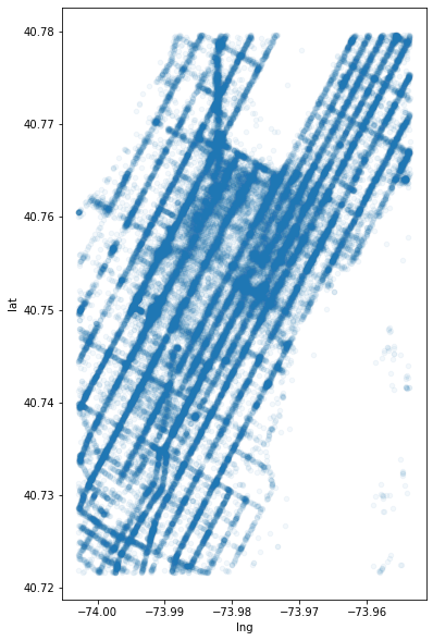
[5]:
df.plot.scatter(x='lng', y='lat', figsize=(6,10), alpha=0.05)
[5]:
<AxesSubplot:xlabel='lng', ylabel='lat'>
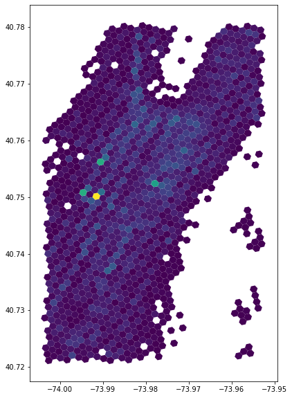
h3_to_geo_boundary()
We can see how many passengers fall into each H3 hexagon.
For now, we will pretend H3-Pandas does not have aggregation functions and perform the aggregations manually
[6]:
dfh3 = dfh3.drop(columns=['lng', 'lat']).groupby('h3_10').sum()
We can now add a H3 hexagonal geometry to each row
[7]:
gdfh3 = dfh3.h3.h3_to_geo_boundary()
gdfh3.head()
[7]:
| passenger_count | geometry | |
|---|---|---|
| h3_10 | ||
| 8a2a10089007fff | 17 | POLYGON ((-73.95877 40.78037, -73.95969 40.780... |
| 8a2a1008900ffff | 110 | POLYGON ((-73.95843 40.77924, -73.95934 40.779... |
| 8a2a10089017fff | 9 | POLYGON ((-73.96032 40.78070, -73.96123 40.780... |
| 8a2a1008901ffff | 97 | POLYGON ((-73.95997 40.77958, -73.96088 40.779... |
| 8a2a1008902ffff | 117 | POLYGON ((-73.95723 40.78003, -73.95814 40.779... |
[8]:
gdfh3.plot(column='passenger_count', figsize=(10, 10))
[8]:
<AxesSubplot:>
h3_to_parent
If we want to perform the analysis on a coarser resolution, we can use h3_to_parent
[9]:
gdfh3_9 = gdfh3.h3.h3_to_parent(9)
gdfh3_9.head()
[9]:
| passenger_count | geometry | h3_09 | |
|---|---|---|---|
| h3_10 | |||
| 8a2a10089007fff | 17 | POLYGON ((-73.95877 40.78037, -73.95969 40.780... | 892a1008903ffff |
| 8a2a1008900ffff | 110 | POLYGON ((-73.95843 40.77924, -73.95934 40.779... | 892a1008903ffff |
| 8a2a10089017fff | 9 | POLYGON ((-73.96032 40.78070, -73.96123 40.780... | 892a1008903ffff |
| 8a2a1008901ffff | 97 | POLYGON ((-73.95997 40.77958, -73.96088 40.779... | 892a1008903ffff |
| 8a2a1008902ffff | 117 | POLYGON ((-73.95723 40.78003, -73.95814 40.779... | 892a1008903ffff |
Again, we pretend that we cannot use aggregation functions and perform the operations manually.
[10]:
gdfh3_9 = gdfh3_9.set_index('h3_09').groupby('h3_09').sum().h3.h3_to_geo_boundary()
gdfh3_9.head()
[10]:
| passenger_count | geometry | |
|---|---|---|
| h3_09 | ||
| 892a1008903ffff | 350 | POLYGON ((-73.95912 40.78149, -73.96123 40.780... |
| 892a1008907ffff | 611 | POLYGON ((-73.95688 40.77891, -73.95899 40.777... |
| 892a100890bffff | 286 | POLYGON ((-73.96340 40.78138, -73.96551 40.780... |
| 892a100890fffff | 686 | POLYGON ((-73.96116 40.77879, -73.96327 40.777... |
| 892a1008917ffff | 544 | POLYGON ((-73.95485 40.78160, -73.95695 40.780... |
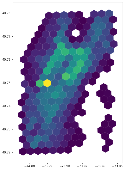
[11]:
gdfh3_9.plot(column='passenger_count', figsize=(10, 10))
[11]:
<AxesSubplot:>

H3-Pandas Extended API: The same workflow, streamlined
The entire above workflow can be performed in one line using aggregation functions of H3-Pandas, namely - h3.geo_to_h3_aggregate - h3.h3_to_parent_aggregate
[12]:
gdfh3_9_alt = df.h3.geo_to_h3_aggregate(10, return_geometry=False).h3.h3_to_parent_aggregate(9)
[13]:
gdfh3_9_alt.plot(column='passenger_count', figsize=(10, 10))
[13]:
<AxesSubplot:>