Unified Data Layers
Original author: Sina Kashuk, modified by Dahn Jahn
This notebook uses the H3-Pandas API to simplify uber/h3-py-notebooks/notebooks/unified_data_layers.ipynb
Summary
One of the applications of hexagons is to be able to combine different datasets with different geographic shapes and forms. In this tutorial we are going through an example of how to bring the US census data, NYC 311 Noise complaints, and Digital Elevation Model to the hexagon aperture and then how to visualize the data to gain insight.
Data
POLYGON: Census Tract Data [Source]
POINT: NYC 311 noise complaints [Source]
RASTER: NYC Digital Elevation Model [Source]
[1]:
pip install h3pandas
Requirement already satisfied: h3pandas in /home/dahn/miniconda3/lib/python3.9/site-packages (0.2.1+5.g23ac830.dirty)
Requirement already satisfied: shapely in /home/dahn/miniconda3/lib/python3.9/site-packages (from h3pandas) (1.7.1)
Requirement already satisfied: pandas in /home/dahn/miniconda3/lib/python3.9/site-packages (from h3pandas) (1.2.5)
Requirement already satisfied: typing-extensions in /home/dahn/miniconda3/lib/python3.9/site-packages (from h3pandas) (3.10.0.0)
Requirement already satisfied: h3 in /home/dahn/miniconda3/lib/python3.9/site-packages (from h3pandas) (3.7.3)
Requirement already satisfied: numpy in /home/dahn/miniconda3/lib/python3.9/site-packages (from h3pandas) (1.21.0)
Requirement already satisfied: geopandas in /home/dahn/miniconda3/lib/python3.9/site-packages (from h3pandas) (0.9.0)
Requirement already satisfied: pyproj>=2.2.0 in /home/dahn/miniconda3/lib/python3.9/site-packages (from geopandas->h3pandas) (3.1.0)
Requirement already satisfied: fiona>=1.8 in /home/dahn/miniconda3/lib/python3.9/site-packages (from geopandas->h3pandas) (1.8.20)
Requirement already satisfied: attrs>=17 in /home/dahn/miniconda3/lib/python3.9/site-packages (from fiona>=1.8->geopandas->h3pandas) (21.2.0)
Requirement already satisfied: certifi in /home/dahn/miniconda3/lib/python3.9/site-packages (from fiona>=1.8->geopandas->h3pandas) (2021.5.30)
Requirement already satisfied: click>=4.0 in /home/dahn/miniconda3/lib/python3.9/site-packages (from fiona>=1.8->geopandas->h3pandas) (7.1.2)
Requirement already satisfied: cligj>=0.5 in /home/dahn/miniconda3/lib/python3.9/site-packages (from fiona>=1.8->geopandas->h3pandas) (0.7.2)
Requirement already satisfied: click-plugins>=1.0 in /home/dahn/miniconda3/lib/python3.9/site-packages (from fiona>=1.8->geopandas->h3pandas) (1.1.1)
Requirement already satisfied: six>=1.7 in /home/dahn/miniconda3/lib/python3.9/site-packages (from fiona>=1.8->geopandas->h3pandas) (1.16.0)
Requirement already satisfied: munch in /home/dahn/miniconda3/lib/python3.9/site-packages (from fiona>=1.8->geopandas->h3pandas) (2.5.0)
Requirement already satisfied: setuptools in /home/dahn/miniconda3/lib/python3.9/site-packages (from fiona>=1.8->geopandas->h3pandas) (49.6.0.post20210108)
Requirement already satisfied: python-dateutil>=2.7.3 in /home/dahn/miniconda3/lib/python3.9/site-packages (from pandas->h3pandas) (2.8.1)
Requirement already satisfied: pytz>=2017.3 in /home/dahn/miniconda3/lib/python3.9/site-packages (from pandas->h3pandas) (2021.1)
Note: you may need to restart the kernel to use updated packages.
[2]:
import pandas as pd
import geopandas as gpd
import h3pandas
import matplotlib.pyplot as plt
Load data
[3]:
# modified data link
ct_data_link = 'https://gist.githubusercontent.com/kashuk/e6e3e3d8fde34da1212b59248a7cc5a8/raw/da3b63c1c0ef4a1c8cc8e10f61455c436a0d0ad9/CT_data.csv'
ct_shape_link = 'https://gist.githubusercontent.com/kashuk/d73342adeccbc65de7a53e19ad78b4df/raw/4300dcb80861d454ecae8f8429166e196779fc21/CT_simplified_shape.json'
noise_311_link = 'https://gist.githubusercontent.com/kashuk/670a350ea1f9fc543c3f6916ab392f62/raw/4c5ced45cc94d5b00e3699dd211ad7125ee6c4d3/NYC311_noise.csv'
nyc_dem_link = 'https://gist.githubusercontent.com/DahnJ/5b77a1d7047412e35e0c1f9ff10ea182/raw/b328c6beb369127081287ac2a17820280d35898b/dem_nyc_xyz.csv'
[4]:
METRIC_COL = 'SE_T002_002' # population density
INDEX_COL = 'BoroCT2010'
Load 311 noise complaints
[5]:
df311 = pd.read_csv(noise_311_link)
Load Census Tract data
[6]:
gdf = gpd.read_file(ct_shape_link).drop(columns='gdf').astype({INDEX_COL: str}).set_index(INDEX_COL)
[7]:
df = pd.read_csv(ct_data_link, usecols=[INDEX_COL,METRIC_COL], dtype={INDEX_COL: str}).set_index(INDEX_COL)

gdf = gdf.join(df)
gdf[METRIC_COL] = gdf[METRIC_COL].fillna(0)
gdf = gdf.loc[~gdf.geometry.isna()]
Load DEM
[8]:
df_dem = pd.read_csv(nyc_dem_link)
Point to hex
[9]:
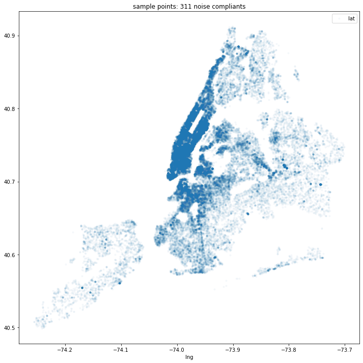
# Visualize the 311 noise complaints points
df311.plot(x='lng',y='lat',style='.',alpha=0.03,figsize=(12,12));
plt.title('sample points: 311 noise compliants');
[10]:
APERTURE_SIZE = 9
[11]:
df311 = (df311
 .assign(count=1)
 .h3.geo_to_h3_aggregate(APERTURE_SIZE))
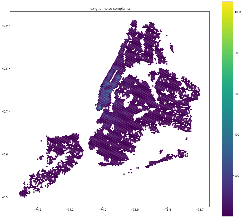
[12]:
df311.plot(figsize=(17, 15), column='count', cmap='viridis', edgecolor='none', legend=True)
plt.title('hex-grid: noise complaints')
[12]:
Text(0.5, 1.0, 'hex-grid: noise complaints')
Spatial smoothing
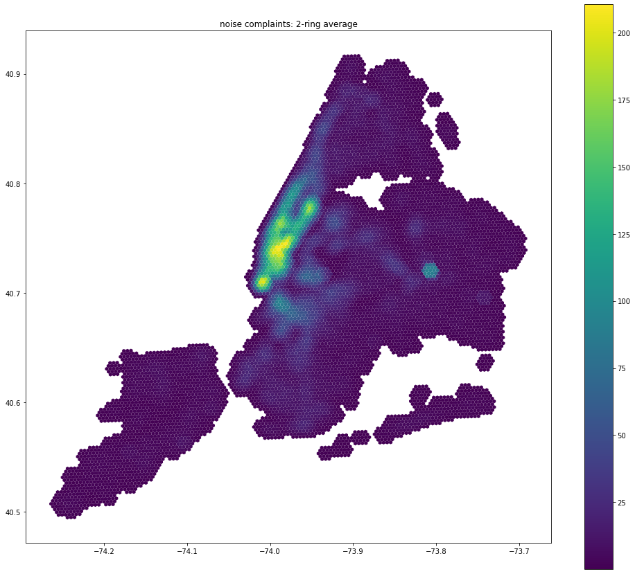
[13]:
k = 2
[14]:
df311s = df311.h3.k_ring_smoothing(k)
[15]:
df311s.plot(figsize=(17, 15), column='count', cmap='viridis', edgecolor='none', legend=True)
plt.title('noise complaints: 2-ring average');
Visualize Census Tract polygons
[16]:
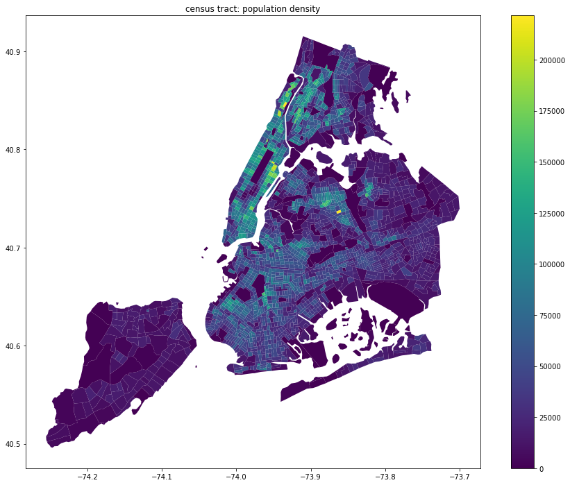
gdf.plot(column=METRIC_COL, cmap='viridis', linewidth=0.05, figsize=(16, 12), legend=True)
plt.title('census tract: population density');
Census polygon to hex
[17]:
APERTURE_SIZE=10
dfh = gdf.h3.polyfill_resample(APERTURE_SIZE)
[18]:
dfh.plot(figsize=(16, 12), column=METRIC_COL, legend=True)
plt.title('hex-grid: population density');

Spatial weighted smoothing
[19]:
coef = [1, .8, .4, .15, 0.05]
[20]:
df_ct_kw = dfh.h3.k_ring_smoothing(weights=coef)
[21]:
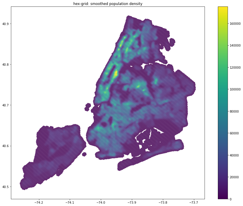
df_ct_kw.plot(figsize=(16, 12), column=METRIC_COL, legend=True)
plt.title('hex-grid: smoothed population density')
[21]:
Text(0.5, 1.0, 'hex-grid: smoothed population density')
Hierarchical re-sampling
Resolution 9
[22]:
df_coarse = df_ct_kw.h3.h3_to_parent_aggregate(9, 'mean')
[23]:
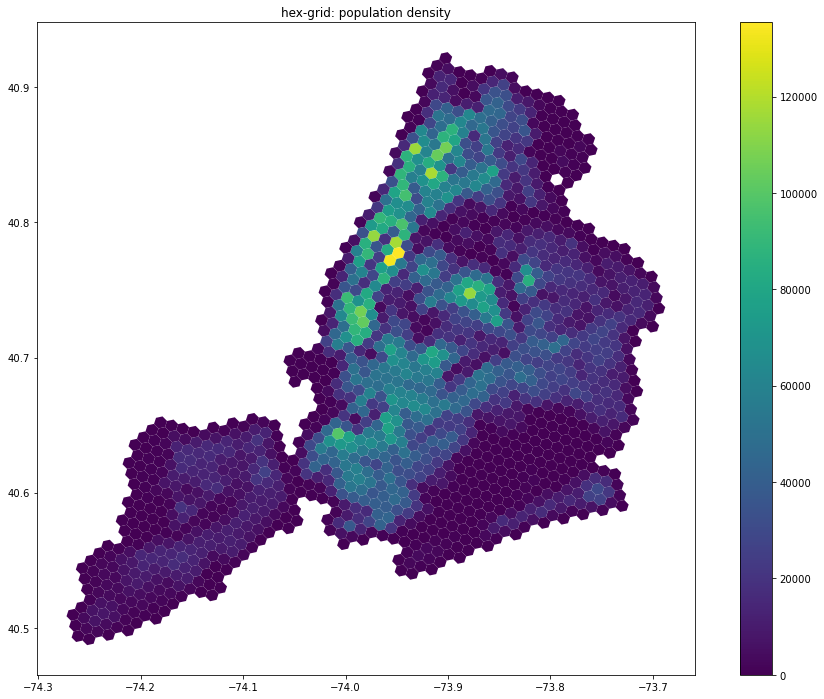
df_coarse.plot(figsize=(16, 12), column=METRIC_COL, legend=True)
plt.title('hex-grid: population density')
[23]:
Text(0.5, 1.0, 'hex-grid: population density')

Resolution 8
[24]:
df_coarse.h3.h3_to_parent_aggregate(8, 'mean').plot(figsize=(16, 12), column=METRIC_COL, legend=True)
plt.title('hex-grid: population density')
[24]:
Text(0.5, 1.0, 'hex-grid: population density')
Raster to hex
[25]:
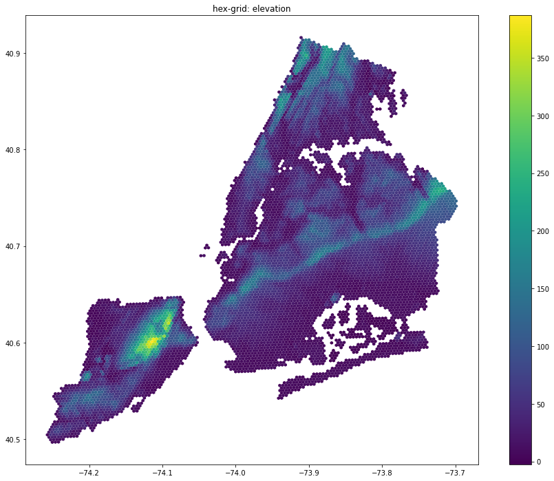
df_dem = df_dem.h3.geo_to_h3_aggregate(9, 'mean')
[26]:
df_dem.plot(figsize=(16, 12), column='elevation', legend=True)
plt.title('hex-grid: elevation')
[26]:
Text(0.5, 1.0, 'hex-grid: elevation')
Unifying data layers
[27]:
dfu = (df_dem
       .join(df311s.drop(columns='geometry'))
       .join(df_coarse.drop(columns='geometry'))
       .rename(columns={METRIC_COL: "population","count":"noise_complaints"}))
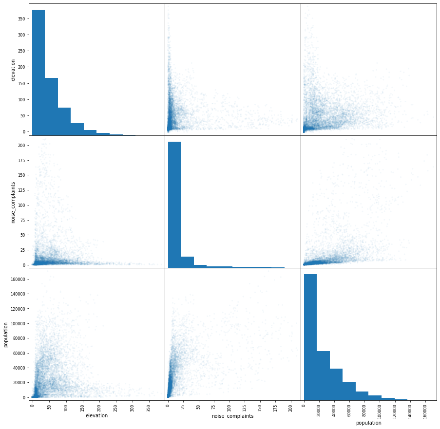
[28]:
pd.plotting.scatter_matrix(dfu, alpha=0.05,figsize=(15,15));
dfu.describe()
[28]:
| elevation | noise_complaints | population | |
|---|---|---|---|
| count | 8047.000000 | 7343.000000 | 8047.000000 |
| mean | 48.874082 | 13.281937 | 24833.451017 |
| std | 49.145254 | 26.843631 | 25614.949764 |
| min | -2.473003 | 0.052632 | 0.000000 |
| 25% | 13.088472 | 2.000000 | 5397.794072 |
| 50% | 32.209505 | 4.315789 | 16142.488019 |
| 75% | 67.886977 | 11.315789 | 37885.947293 |
| max | 386.767609 | 210.578947 | 170595.715931 |